Statistical analysis

For statistical nanoindentation (SNI) results [12] or for statistical analysis of the mechanical property values distribution, it is possible to use histograms or to use a cumulative distribution. According to Tuinukuafe et al., SNI may be ineffective for measuring the mechanical properties of individual phases in a microstructure if they are not prolific enough to exhibit a continuous indent response [12]. This conclusion can be directed linked to the question of the indentation length scales (see https://tridimap.readthedocs.io/en/latest/mapping.html#indentation-length-scales).

Probability density function (PDF)

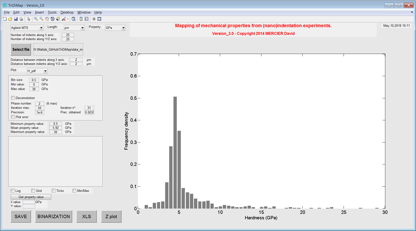
Figure 23 Histograms of hardness values

Using histograms is really interesting for the visualization point of view with a common pattern, like the bell–shaped curve. Such a curve is known as the “normal distribution” or the “Gaussian distribution”. For an homogeneous material, only 1 peak is expected and for an heterogeneous material, a peak per phase can be expected. In this last case, intermediate peaks between phase peaks can be observed when interfaces are not spatially negligible. The drawback of this plot is the user-dependence of the bin size and thus of the distribution shape (i.e. peak intensity). Indeed, the shape of the distributions is bin size dependent, while this bin size (e.g. 0.5GPa or 3GPa) is defined arbitrary by the user. This issue is well known in the literature and is a little bit discussed in this presentation [5] and this paper [4]. The shape of the distributions is also bin step dependent. In other words, if the the histogram starts from an odd or an even value, the distribution is different.

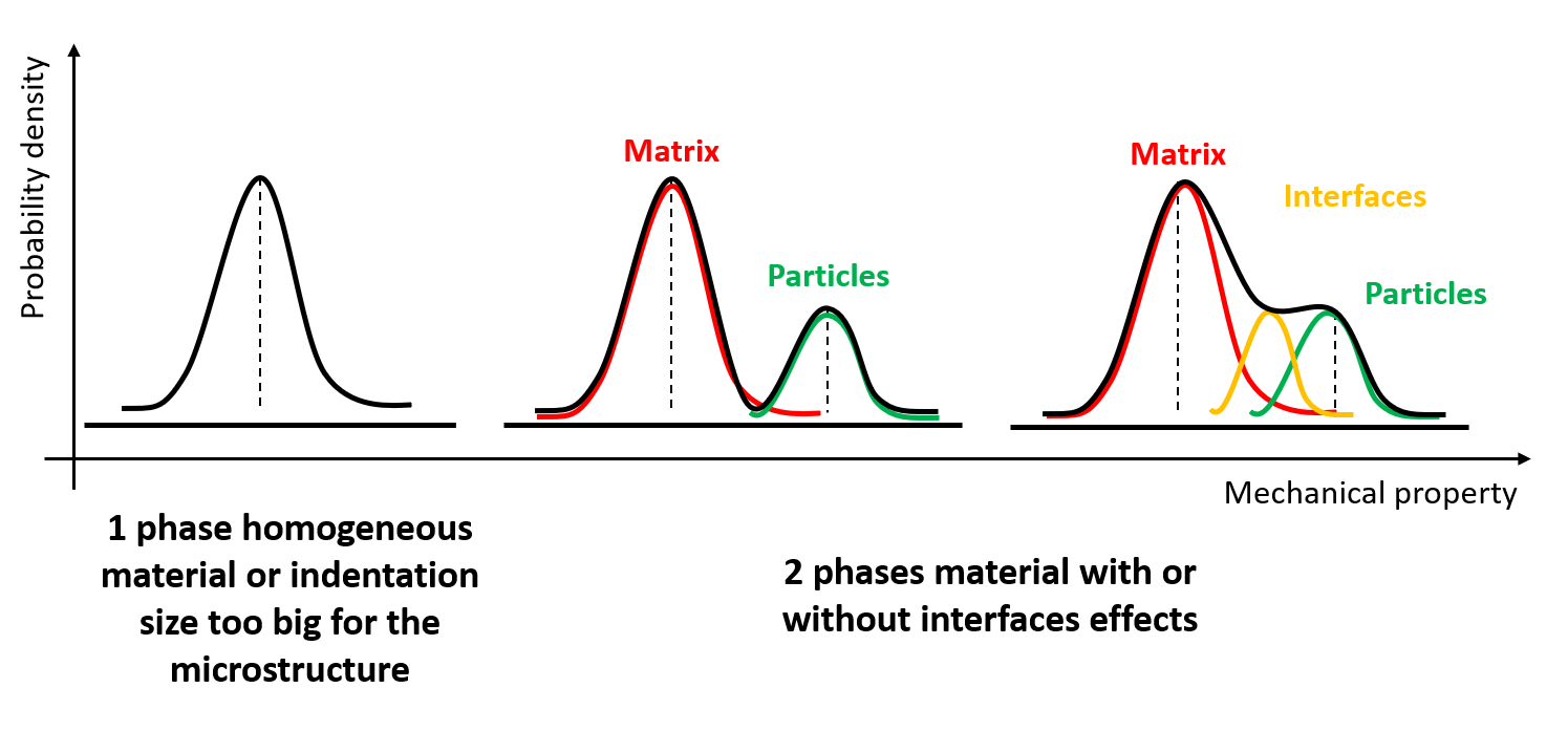
Figure 24 Example of different fitted histogram distribution schematized as a function of the specimen

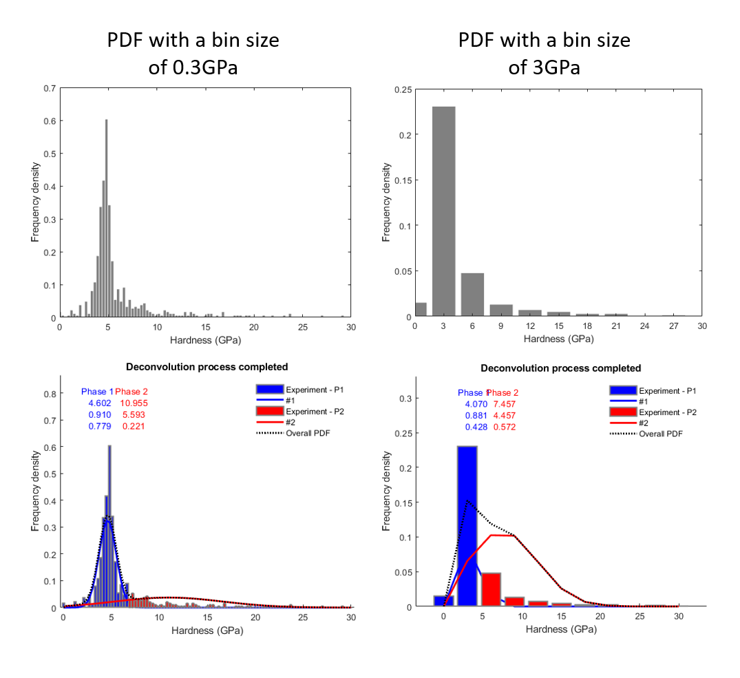
Figure 25 Effect of the bin size definition on the distribution shape

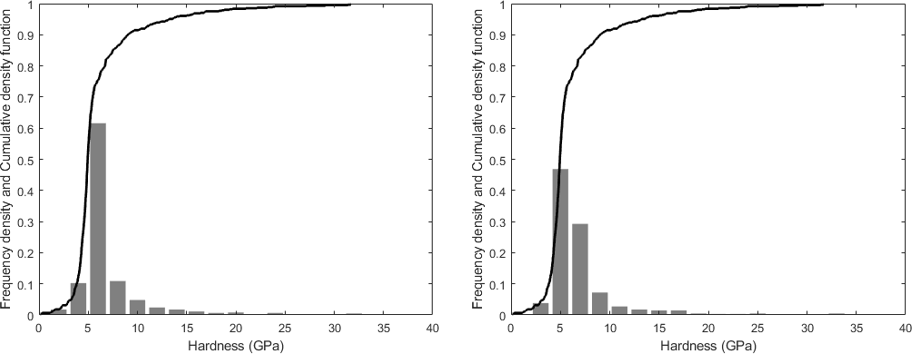
Figure 26 Effect of the bin step on the distribution shape: the histogram start from 0GPa on the left and from 1GPa on the right, using the same bin size of 2GPa.

The next step is to fit this distribution using a probability density function. Such mathematical approach is very well defined in the literature [6], [10] and [3]. It is worth to note that the result obtain after deconvolution (average values and standard deviations for each peak) is dependent of the bin size. A solution to avoid user definition of the bin size is to use the Freedman–Diaconis rule of thumb, which gives an estimation of the bin size after calculation the interquartile (IQR) range of the data [2]. To activate this option, check the box for ‘Auto Bin Size’ on the GUI.

(3)\[\text{Bin Size} = \frac{2*IQR}{n^{\frac{1}{3}}}\]

With \(n\) is the number of observations in the sample.

The Matlab function used to calculate the interquartile range of the data is: iqrVal.m

Another rule of thumb is to use between 6 and 20 bins in a histogram.

The Matlab function used to plot the distribution of mechanical property values using histogram is: pdfGaussian.m

The Matlab function used to fit using a probability density function and to process the deconvolution is: TriDiMap_runDeconvolution.m

This last function has been extensively inspired by the work of Němeček J. et al. [7], [8] and [9].

An example of fitting and deconvolution process is given in the following figure, followed by another example of decomposition process leading to phase mapping and plot of corresponding cumulative distributions.

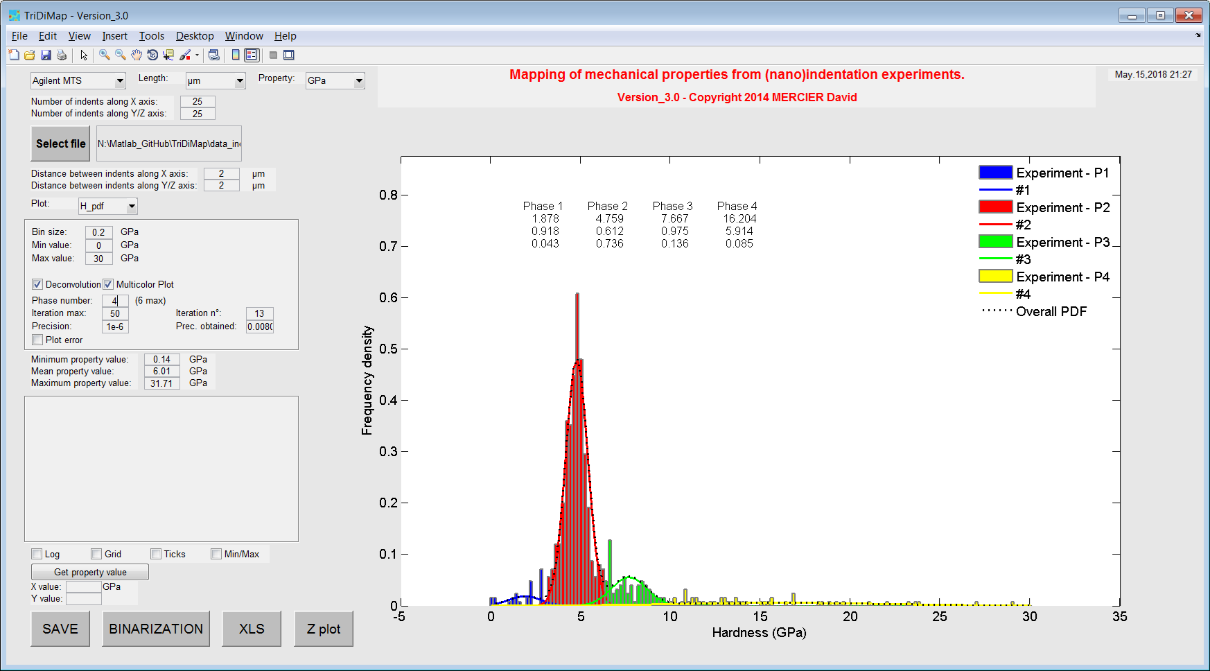
Figure 27 Histograms of hardness values with Gaussian PDF after fitting and deconvolution step

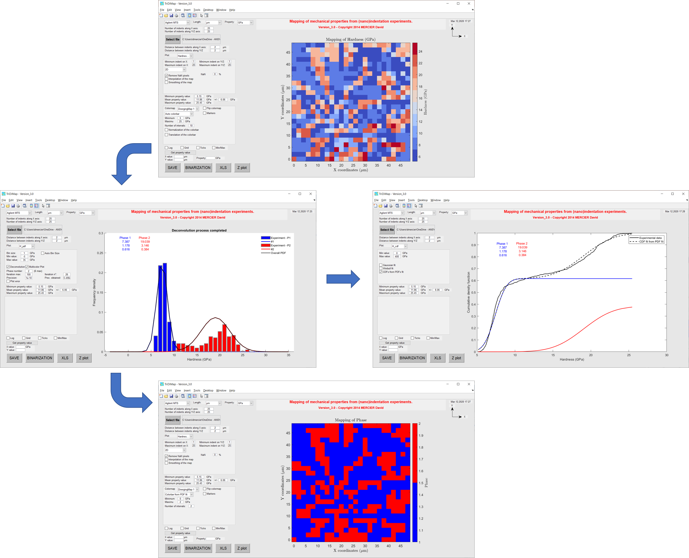
Figure 28 Phase map and cumulative distributions of each phase resulting from decomposition step

Note

Effect of the interphase can be considered and could be implemented in this toolbox [1].

Note

The choice of the bin size could be defined as an automatic calculation, based on the number of phases, the number of data and the minimum of peak intensity…

When data are noisy due to experimental artefacts (e.g. surface contamination, interfaces effect or interesting phase inside the sample…) for example, with very high or very low mechanical property values, it is always possible to cut the signal, by setting manually (on the GUI) the extrema. This operation can be seen as an arbitrary cleaning, but careful with a fitting process, which gives different mean values, given peak shapes or peak number modification.

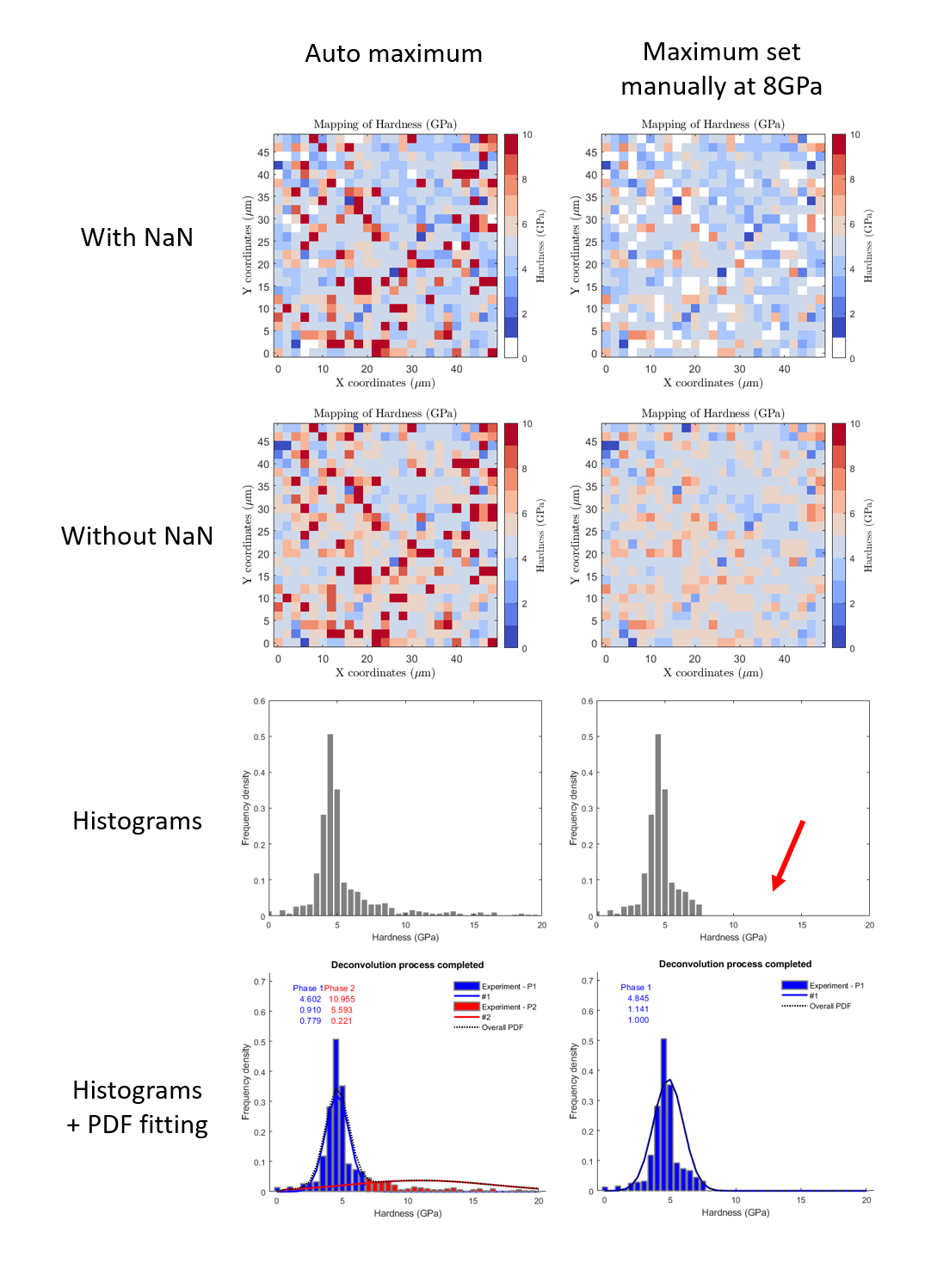
Figure 29 Example of manually saturated indentation data, with a comparison between automatic maximum and a maximum set to 8GPa

Note

Sometimes the fit does not converge, just restart the fitting process… or change a little bit the bin size.

Cumulative density function (CDF)

The cumulative distribution of mechanical property is much better than an histogram plot (no bin size dependency). But, it is much more difficult to decompose and in this toolbox, only Gaussian and Weibull fitting are proposed, which is only interesting for an homogeneous material. The Weibull function is from the PopIn toolbox [11].

The Matlab function used to plot the cumulative distribution of mechanical property values is: cdfGaussian.m

The Matlab function used to fit the cumulative distribution with a Weibull function is: TriDiMap_Weibull_cdf.m

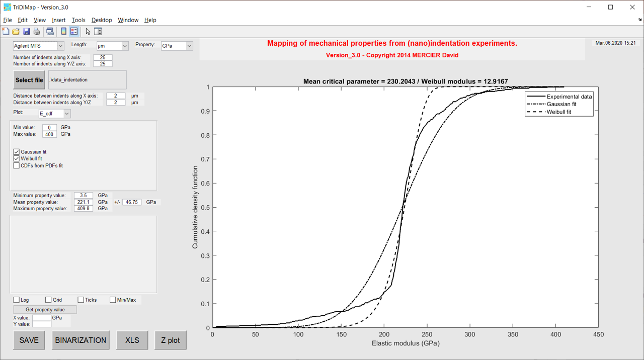
Figure 30 Cumulative distribution of elastic modulus values with Gaussian and Weibull fitting

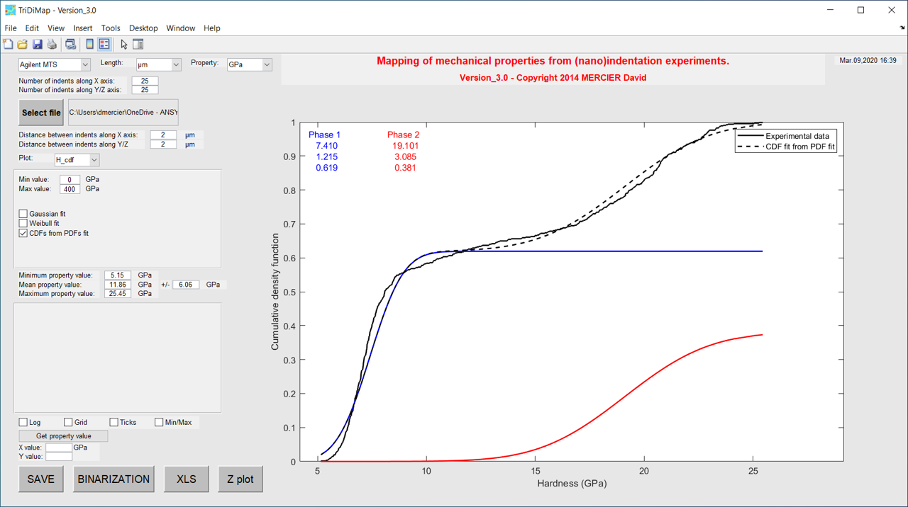
Figure 31 Cumulative distribution of elastic modulus values with cumulative distributions for each different phase

References

[1]

Čech J.et al., “Approche statistique pour identifier les propriétés mécaniques des phases individuelles à partir de données d’indentation” (2017).

[2]

Freedman D. and Daconis P., “On the histogram as a density estimator:L2 theory” (1981).

[3]

Haušild P. et al., “Determination of the individual phase properties from the measured grid indentation data” (2016).

[4]

Hrbek V. and Koudelková V., “Grid Indentation and Statistic Deconvolution: Limitations and Accuracy” (2017).

[5]

Mercier D. et al., “Combined techniques for the characterization of an electrodeposited Nickel coating with embedded SiC particles: from microstructure to local mechanical properties” (2016).

[6]

Němeček J., “Nanoindentation of heterogeneous structural materials”, PhD thesis (2009).

[7]

Němeček J., “Probability density function 1.0” (2010).

[8]

Němeček J., “Probability density function 2.1” (2010).

[9]

Němeček J., “Deconvolution algorithm 3.0” (2010).

[10]

Němeček J. et al., “Micromechanical analysis of heterogeneous structural materials” (2013).

[11]

Mercier D.et al., “PopIn documentation”.

[12] (1,2)

Tuinukuafe A.et al., “On the Role of Continuity in Statistical Nanoindentation of Composite Microstructures”.